July 13, 2022

What to expect when you’re expecting a better climate model

P#7 •  ePUB    •    PDF    • 17 min  •   comments 

If we build a gigantic supercomputer, ask it the ultimate question, and receive a single number as an answer, what have we learned? Without context, not much. A single number, whether it is 42, as in The Hitchhiker’s Guide to the Galaxy,¹ or 3°C for Earth’s climate sensitivity, doesn’t mean much unless we know how it was calculated and what its uncertainty is.

This provides a nice segue to the recent blog discussion about a concerted international effort to build a climate model with a 1-km (k-scale) horizontal grid.² That would be a big jump from the current generation of climate models, which typically use a 50-km grid. The common expectation is that a million-fold increase in computer power available for modeling will lead to a quantum leap in our predictive capabilities, thus better informing policy-makers. The headline of a recent Wall Street Journal article, “Climate Scientists Encounter Limits of Computer Models, Bedeviling Policy”, reflects this sentiment.³

To what extent can better climate models inform policies, and exactly what policies can they help inform? The phrase “actionable predictions” is frequently used in this context, but often without elaboration. How much improvement in predictions can we expect from much better climate models of the future? Will they reduce the error bar by 10%, 50% or 90%? It turns out that our current models have something to say something about that.

Limits and uncertainties of climate prediction

From our familiarity with weather forecasts, we know there are limits to weather prediction. We don’t expect forecasts to be accurate beyond about a week. That’s because we have imperfect knowledge of the initial condition for a weather forecast. Small errors in the initial condition grow exponentially over time leading to large errors in the forecast after several days. This property of chaos, known as the Butterfly Effect, limits weather prediction to about two weeks. Even a perfect weather model cannot predict beyond this limit.

Is there a corresponding limit to climate prediction? The usual answer is that the Butterfly Effect does not apply to climate prediction because we are not predicting individual weather events but the statistics of future weather. That’s technically true, but what happens to the Butterfly Effect beyond two weeks? The error associated with the Butterfly Effect eventually stops growing and saturates in amplitude, morphing into stochastic uncertainty or internal variability in climate prediction. Since we can never be rid of it, we could call it the Cockroach Effect. Even that may be misleading because we could reduce roach numbers with pesticides but the stochastic uncertainty is fundamentally irreducible—it will persist even in a perfect climate model. We can estimate the amplitude of stochastic uncertainty by carrying out climate predictions with different initial conditions.

You may not have heard much about stochastic uncertainty because it’s not important when predicting global average temperature, which dominates popular discussions of global warming. Predicting societal impacts, or even tipping points, requires prediction of regional climate, which is where stochastic uncertainty becomes important. (If ice sheet instabilities and/or oceanic overturning circulation instabilities turn out to be more important on centennial timescales than currently believed, that will likely increase the amplitude of global chaotic/stochastic uncertainty.)

There are two further uncertainties in climate prediction, and they do affect global average temperature.⁴ The next is scenario uncertainty. This arises from unpredictable human actions that determine the scenario of future carbon emissions and thus the magnitude of the resulting global warming. This uncertainty cannot be characterized probabilistically and is scientifically irreducible. Even a perfect climate model will exhibit this uncertainty—only human actions (including technological developments) can reduce it. We estimate this uncertainty by carrying out predictions with different emission scenarios.

The third uncertainty in climate prediction is model uncertainty which arises from structural differences in the representation of small-scale processes like clouds in climate models. Since these processes occur on scales too fine to be resolved by the coarse spatial grids of the climate, they are represented using approximate formulas known as parameterizations. The errors in these parameterizations lead to spread in predictions using different models. This is the only scientifically reducible error in climate prediction. Using a model with a finer grid, such as a k-scale model, can decrease this uncertainty because fewer processes will be poorly represented. We estimate this uncertainty by carrying out predictions with climate models using different parameterizations.

Meta-prediction: Predicting the future of prediction

Analyzing the partitioning between the three different types of uncertainty in our current models allows us to calibrate our expectations for better models. Two important measures of how quickly the globe might warm are transient climate response (TCR) and equilibrium climate sensitivity (ECS). These two measures are basically rough estimates of how much warming doubling of carbon dioxide will cause by the end of this century and over many centuries, respectively. As we see in Figure 1, the spread in these measures has not decreased as the models have gotten “better” over the years. If anything, the ECS spread has increased in recent decades. Figure 2 shows the multi-model average of the global warming projected for three different emission scenarios. The error bars show the model uncertainty for each scenario. Note that the scenario uncertainty is comparable to, or larger than, the model uncertainty.

New let us perform a thought experiment. Suppose we have a future IPCC Assessment Report AR(k) based on a single k-scale model. That means we have a model that predicts climate out to year 2100 using a 1-km spatial grid. As we see in Figure 1, we would have an additional estimate each for TCR and ECS, respectively. But without multiple independent k-scale models, we cannot assess the model uncertainty, i.e., the spread in TCR or ECS. We’d have no way of knowing if the AR(k) estimates are superior in any sense.

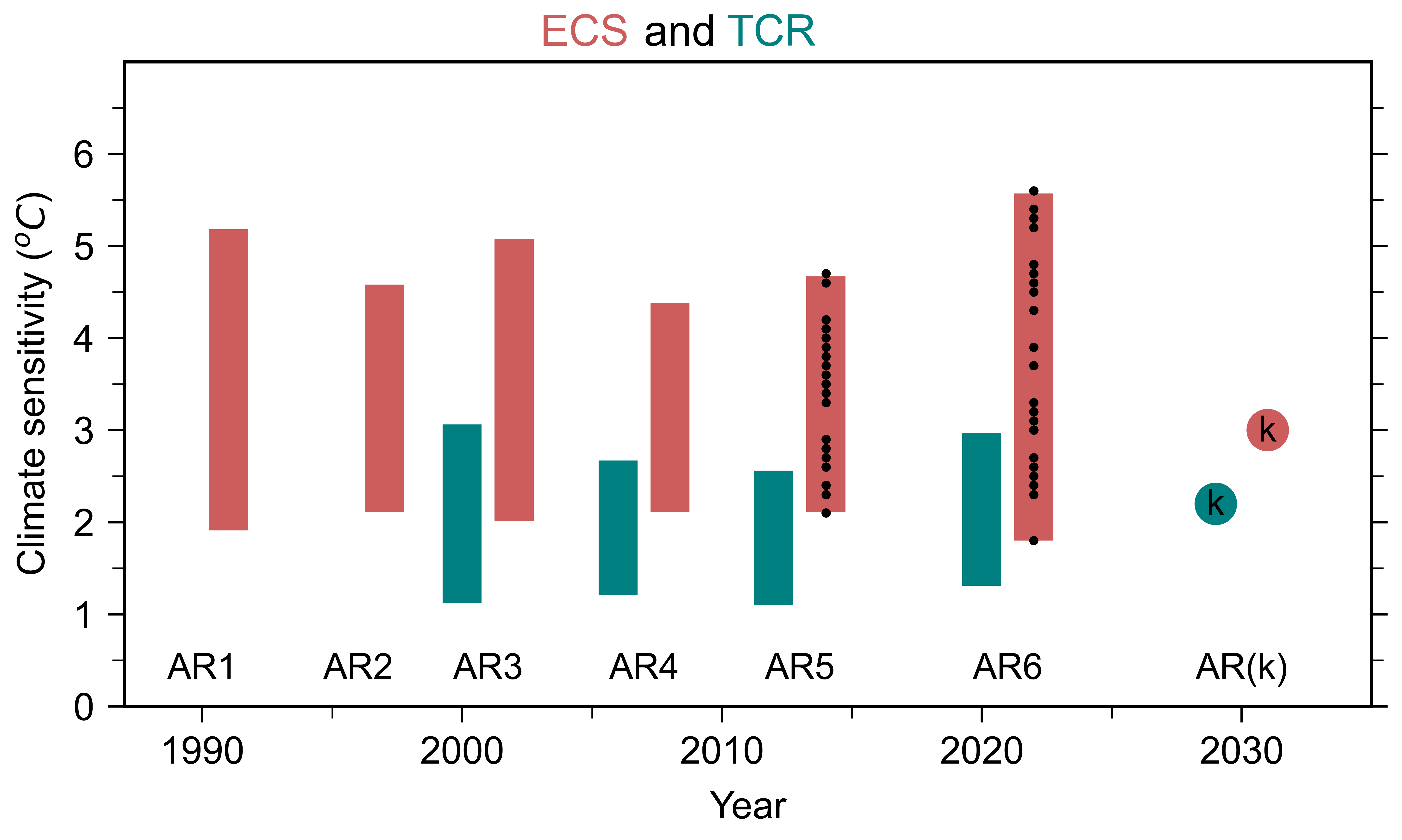
Figure 1. Model-simulated values of equilibrium climate sensitivity (ECS; red) and transient climate response (TCR; teal) from successive IPCC Assessment Reports from AR1 to AR6. The bars show the spread of values estimated by different models, with black dots showing individual model values for AR5 and AR6. The solid circles show ECS and TCR value assessed for a hypothetical IPCC AR(k) in 2030 using a single k-scale model. [Adapted from Meehl et al. (2020)]⁵

Let us be optimistic and assume further that we are able to afford to run many independent k-scale models for the hypothetical IPCC AR(k) and the spread between these models has reduced by a factor of 2 (say). As we see in Figure 2, the spread in predicted warming by 2100 for different scenarios will become the dominant uncertainty, and will persist even if we had the perfect climate model. Mitigation policy decisions will not benefit very much from reduced model uncertainty or narrower estimates of climate sensitivity, because scenario uncertainty dominates. When it comes to predicting how much the globe will warm by the end of the century, the biggest uncertainty is us.⁶

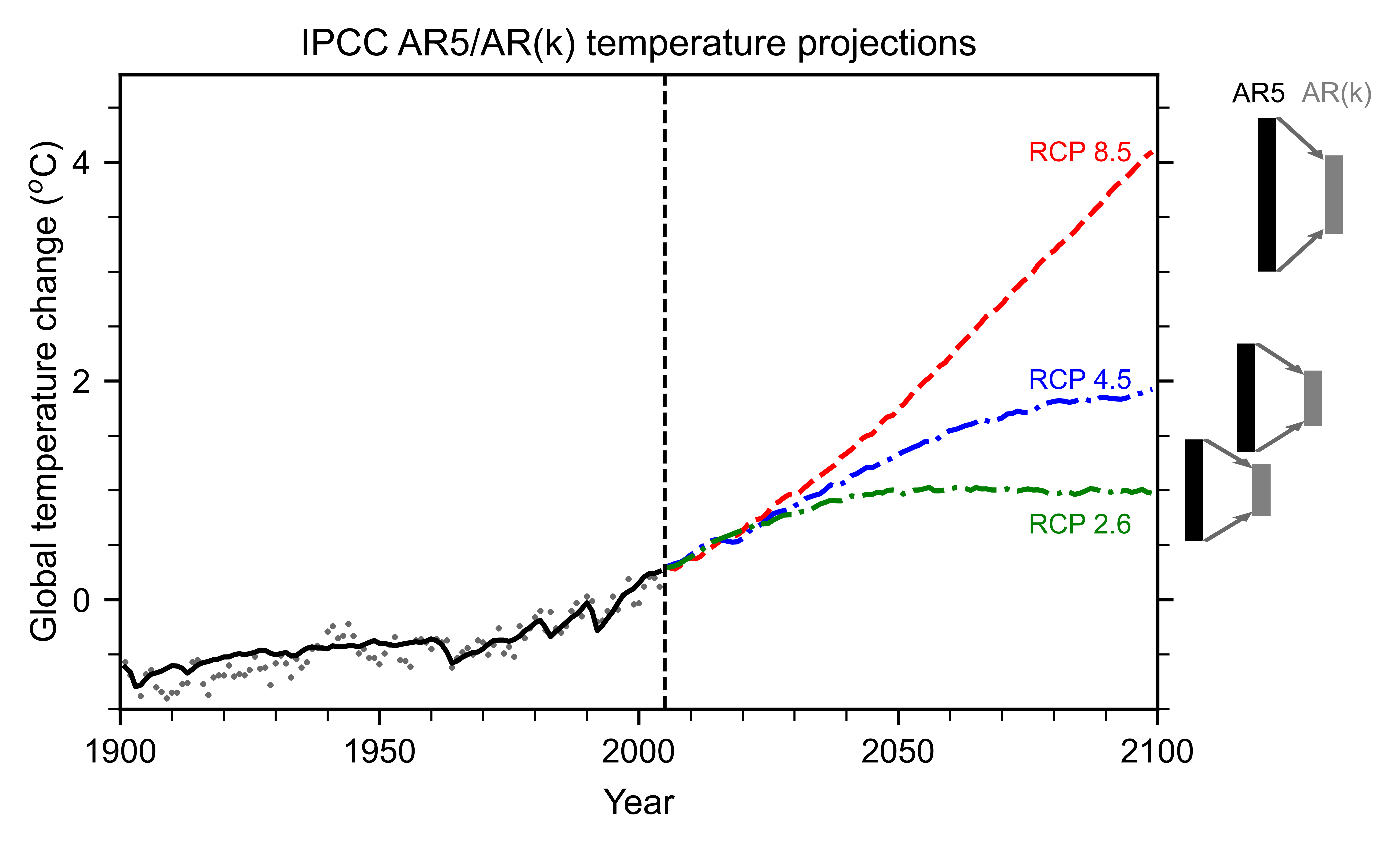
Figure 2. IPCC AR5 multi-model average prediction of global-average surface temperature for three emission scenarios, high-end (RCP8.5; red), medium (RCP 4.5; blue) and low-end (RCP 2.6; green). The black bars show the AR5 model uncertainty, or the spread amongst models; the gray error bars show what it would look like if the spread was reduced by a factor of 2 by better models in the hypothetical AR(k). (AR5 projections are shown rather than AR6, because AR6 uses model weighting to shrink its larger error bars to resemble AR5 anyway.) [Adapted from Knutti and Sedlaček, 2013]⁷

The dominance of scenario uncertainty for centennial prediction of global temperature is illustrated more vividly by the evolution of the uncertainty partitioning over time (Figure 3a). Scenario uncertainty grows monotonically but is relatively small for the first decade-and-a-half of the prediction, while model uncertainty peaks around that time. Therefore, reducing model uncertainty would have the biggest (fractional) benefit for global predictions on decadal timescales.

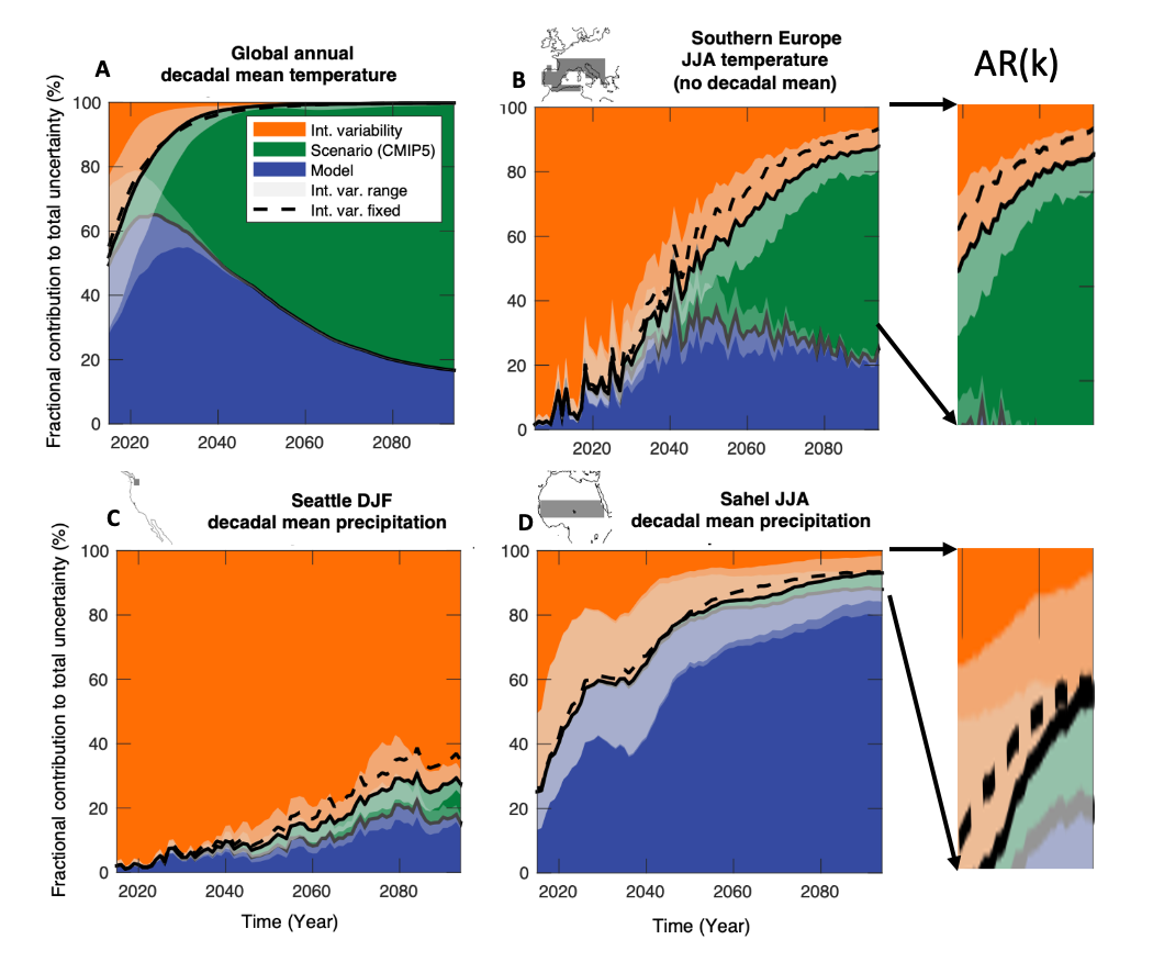Figure 3. Partitioning of the uncertainty (stochastic/internal-orange; scenario-green; model-blue) for decadal-average model predictions of: A. Global-average surface temperature; B. summer (Jun-Jul-Aug) temperature over southern Europe (no decadal average); C. winter (Dec-Jan-Feb) precipitation in Seattle, Washington (USA); D. summer (Jun-Jul-Aug) rainfall over the Sahel region of Africa. The lighter shading denotes the higher-order uncertainty in model estimates of stochastic internal variability. If we had a perfect model, the model uncertainty fraction (blue) would vanish, but other uncertainties would remain. The two “blow-ups” on the right illustrate this for a hypothetical AR(k) with greatly reduced model error. [Adapted from Lehner et al., 2020]⁸

Improved prediction of just the global averages is not very useful for assessing societal impacts, which depend on the details of regional climate change. Say we are interested in predicting summer temperatures in southern Europe. The dominant uncertainty is associated with the emission scenario (Figure 3b). Model error accounts for only 30% of the prediction uncertainty. That means even a perfect model would reduce the total uncertainty by no more than 30%. (The regions where we can expect model improvements to provide the most “bang for the buck” are those where model error is the dominant uncertainty and emission scenarios are the second-most important uncertainty, such as over the Southern Ocean.)

Next, we consider two regions with contrasting behavior for regional precipitation prediction: the rainy city of Seattle in Washington state, USA and the dry Sahel region of Africa (Figures 3c,d). In both regions, the scenario uncertainty fraction is small, but the model uncertainty fraction is quite different.

If we are interested in predicting Seattle rainfall for the end of the century, current models tell us that better models may not make much of a difference—unpredictable and irreducible stochastic uncertainty accounts for over 70% of the total, meaning that rainfall changes will remain hard to predict (Figure 3c).

Predicting Sahel rainfall for the end of the century tells a different story (Figure 3d). Spread among different models plays a dominant role in the uncertainty. This is the manifestation of a common problem in climate modeling—the large biases in the simulated climate in certain regions. The focus on global average temperature often masks these large regional biases. Higher resolution models would definitely be helpful in reducing these biases.

What if k-scale models were able to substantially reduce the model spread in the Sahel region? Figure 3d suggests that this would cause internal variability to become the dominant uncertainty in the Sahel region. With a better model, Sahel rainfall may still be mostly unpredictable on centennial timescales, but we will be able to say that with more confidence and a much smaller error bar.

We have considered changes in time-averaged temperature and rainfall. But extremes in temperature and rainfall are also very important because they can have severe impacts. Currently, our coarse-resolution climate models cannot predict rainfall extremes very well, because rain is determined by small-scale air motions and microphysical processes. With finer resolution and parameter tuning, k-scale models should be able to do a better job of simulating these extremes in our current climate. The extent to which k-scale models can better predict how rainfall extremes will change in a future climate is an open question—it will depend upon how big a role uncertainties in the still unresolved microphysical processes will play.

Deconstructing the promise of k-scale

We have outlined what we might expect from better climate models with regard to reducing uncertainty. Now we consider the two recent Nature Climate Change articles about k-scale modeling that triggered the blog discussions, one about the atmosphere and the other about the ocean. Their titles are:

1. Ambitious partnership needed for reliable climate prediction (ATM)⁹

2. The small scales of the ocean may hold the key to surprises (OCN)¹⁰

As is often the case in climate discussions, ambiguities in language can lead to a mismatch between what the public thinks that science can deliver and what the science is actually capable of delivering. Therefore, it is worth deconstructing what these articles actually say about the benefits of k-scale modeling.

For example, consider the phrase “climate prediction”, which appears in the title of the ATM article. Climate scientists use this phrase even for predictions of the average weather for the next season, because climate is the average weather. But the public is more likely to associate “climate prediction” with IPCC and predictions of global warming extending to the end of the century (absent additional qualifiers like “seasonal climate prediction”). This conflates two very different types of prediction: one where initial conditions provide the signal and another where they become the noise.

The ATM article talks about reliable predictions from “daily weather to decadal variability, conditioned by global warming trends”. Reliability cannot be assessed for centennial timescale predictions, due to lack of data. Therefore, the article seems to be implicitly focusing more on reducing model biases to improve predictions of El Niño and other phenomena up to the decadal timescale. This is the timescale where reducing model uncertainty will be most beneficial in improving global predictive skill (Figure 3a).

K-scale models should be able to better predict the future statistics of local extreme events on shorter timescales because they can resolve fine-scale fluid motions associated with cloud processes. On longer timescales, however, errors in other non-fluid components of the climate system—such as microphysical processes in clouds or the carbon cycle—will play an increasing role. The direct benefit of k-scale modeling in reducing the uncertainty of centennial climate predictions would therefore be more limited. There would still be the indirect benefit of increasing our confidence in such long-term climate predictions.

The OCN article, on the other hand, does not even mention predictions and instead talks about projections, implying longer timescales. (The title actually refers to “surprises”, which is quite the opposite of prediction.) Higher resolution can improve ocean simulation in critical regions that affect possible tipping point behavior associated with Atlantic ocean circulation. Current comprehensive climate models do not exhibit tipping points, but it is possible that higher resolution models could exhibit more nonlinear or threshold behavior. The suggestion, therefore, is that current models could be underestimating oceanic internal variability.

Despite their contrasting views on prediction, the common thread in both articles is the utility of higher spatial resolution to reduce biases in models and improve our understanding of the climate system. This will improve our confidence in climate predictions but should we expect it to significantly reduce the spread in predictions?

Our everyday experience with prediction comes from weather forecasts. We expect that a better weather model using more powerful computers will make predictions with a smaller “error bar”. This error bar, which we can calculate using past observations, has indeed decreased over time with better weather models.

Climate prediction is fundamentally different. Since centennial-scale global warming is an unprecedented event, we cannot use observational statistics to compute its error bar.¹¹ Therefore, the same climate models that make predictions are also used to estimate the spread or the “error bar” associated with their predictions. Better climate models can give us more knowledge because more processes are added or represented better, but the associated error bar could be larger. More knowledge may not always lead to more certainty!¹²

One model to rule them all?

Contrary to some media headlines, it’s not the lack of better models that bedevils climate mitigation policy, but the lack of political will. More computing power for models can help improve the skill of short-term (seasonal-to-decadal) predictions, but that would not be relevant to climate policy.

The understanding gained from better short-term predictions can help improve models used for long-term prediction by reducing biases, especially in their precipitation simulations. Depending upon the relative strengths of internal variability and model error in each region, these improvements may or may not significantly reduce the quantified uncertainty of long-term prediction (Figure 3). Nevertheless, better models would increase our confidence in long-term predictions and provide a sounder basis for climate adaptation policies.

The ATM article recommends spending certain dollar amounts to support k-scale modeling, but doesn’t spell out exactly how they should be spent. Should the money be used to build a giant supercomputer associated with a single, international modeling center, or should it be distributed among many centers? Let us consider the former option, i.e., creating the climate-equivalent of CERN, the international facility dedicated to experimental particle physics with an order of magnitude more resources than any national facility:

• A single k-scale CERN for centennial climate prediction: This would be a bad idea. Such a Climate-CERN will gain de facto authority because its model will be considered “better” and its climate prediction will be considered official. Since it will contribute only one data point in Figure 1, there’ll be no way to estimate the error spread. Of course, the Climate-CERN could develop multiple model structures to estimate the spread. But to do that well, it may require at least 10-20 different model structures. It would be better for these model structures to be developed at separate modeling centers under independent management. (As anyone who has worked at a modeling center could tell you, human factors affect the choice of model structure as much as scientific factors.) Collaboration and standardization of coding structure between multiple modeling centers would certainly be beneficial. Sharing a single supercomputer to run independent models would also be fine.

• A single k-scale CERN for seasonal-to-decadal prediction: This could be a good idea, serving as a proof-of-concept for the touted benefits of k-scale modeling. The goals and performance benchmarks of such a SeaDec-CERN would need to be clearly defined, to avoid “mission creep”. Limiting predictions to shorter timescales would also prevent the dilution of computing resources. The short-term predictions would provide public benefits, but may not help mitigation or adaptation policies. A SeaDec-CERN may also gain authority because it has a “better” model, but there’s a self-correcting mechanism. We’ll know soon if the k-scale El Niño forecasts are substantially better than competing models with fewer resources. If they are not, which is quite possible, then SeaDec-CERN will lose its authority. If the forecasts improve substantially, then the knowledge gained can help reduce biases in long-term climate prediction models.

• Black swans, unknown unknowns, and fundamental research: We have focused so far on what to expect from better models. But what is unexpected—the “surprises” alluded to in the OCN article—could be more interesting. We know that our climate models are imperfect representations of the complex climate system. In our climate future, we may encounter a black swan event that was never anticipated or cross a tipping point that was unpredictable. Having the most comprehensive model, but not necessarily the most complex model, would help us be better prepared when we encounter unknown unknowns. A good example is the discovery of the Antarctic ozone hole.¹³ Without good atmospheric chemistry models that were already available, it would have taken us much longer to understand the mechanism of the ozone hole. Even though these models never predicted the emergence of the ozone hole, they could be modified to predict its future evolution. Model development for the sake of better understanding is typically considered fundamental research, because it does not provide “actionable predictions”. Rather than be obsessed with predictions, one can argue that it is important for society to support fundamental climate research as a form of planetary defense—on par with, or even exceeding, other big science projects like space-borne telescopes, planetary missions, and particle accelerators.

Note: As noted in a blog comment, an international center for long-term climate prediction that builds a model at current spatial resolution may be justified for a very different reason. Scientists from developing countries lack the resources to build and use climate models to answer questions that are most relevant to them. Having an international climate modeling center dedicated to their needs would be a great idea!